Backward-in-time, Finite-Size Lyapunov Exponents and Orientations of associated eigenvectors
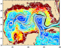
The maps of Backward-in-time, Finite-Size Lyapunov Exponents (FSLEs) and Orientations of associated eigenvectors are computed over 30-year altimetry period and over global ocean within the SALP/Cnes project in collaboration with CLS, LOcean and CTOH. These products provide the exponential rate of separation of particle trajectories initialized nearby and advected by altimetry velocities. FSLEs highlight the transport barriers that control the horizontal exchange of water in and out of eddy cores.
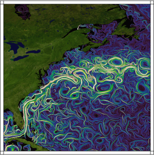
Large FSLE values (in clear colors on the figure) identify regions where the stretching induced by altimetry-detected mesoscale velocities is strong. Large FSLE values are typically organized in convoluted lines encircling (sub-)mesoscale filaments. Ridges of FLSE are often in good agreement with filaments of biogeochemical tracers (Ocean Color, Sea Surface Temperature,...) affected by horizontal advection.
The observed filaments in tracer images correspond to stable trajectories (contraction) of the flow where streching is strong. When computed using a backward-in-time advection, the FSLE also show convoluted lines encircling sub-mesoscale filaments that are often in good agreement with the main structures of biological tracers distribution.
Even if few studies have been done on eigenvectors associated to FSLEs, it is known that the orientation of eigenvectors are also in good agreement with the geophysical tracer gradient orientation. Moreover, it is more robust to compare angles than filaments positions. Thus this variable is proposed in the products to encourage its use in future studies.
Methodology
Backward-in-time FSLEs ridges approximate the so-called Lagrangian Coherent structures which are the generalization of stable hyperbolic trajectories of time independent flow. They are defined as the larger eigenvalues of the Cauchy-Green strain tensor of the flow map. FSLEs are strongly linked with the exponential rate λ of separation of two neighboring particles during a time advection t:
| λ = t -1 . log(δf/δ0) |
where δ0 (resp. δf) is the initial (resp. final) separation distance which are fixed before computation (see below).
The method was initiated by F. d'Ovidio, LOcean. The products are delivered via the Aviso+ website. The source code is also distributed open source if you intend to apply your own parameters (see code delivery).
For version DT2024, the code has been actualized in https://py-eddy-tracker.readthedocs.io/en/stable/python_module/07_cube_manipulation/pet_fsle_med.html (Copyright 2019, A. Delepoulle & E. Mason)
The FSLE calculation (values and structures) has been shown to be robust against random noise which mimics unresolved scales. See Cotté et al., 2011, p. 224 for details.
References:
- d'Ovidio F., V. Fernández, E. Hernández-García, C. López, 2004, “Mixing structures in the Mediterranean sea from Finite-Size Lyapunov Exponents”, Geophys. Res. Lett., 31, L17203.
- Cotté C., F. d'Ovidio, A. Chaigneau, M. Lévy, I. Taupier-Letage, B. Mate, C. Guinet, 2011, "Scale dependant interactions of Mediterranean whales with marine dynamics", Lym. Ocean. 56(1), 219-232.
FSLE is a scalar that is computed at a given location. Seeding a domain with particles initially located on a grid leads to the computation of discretized fields.
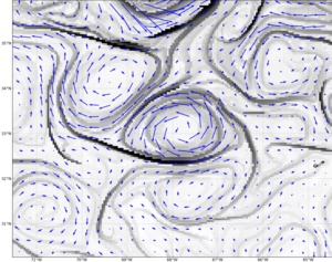
Because they are computed on a finer grid than mesoscale altimetry velocity fields, the Lyapunov Exponents can underline sub-mesoscale structures. Moreover as velocity fields are time dependant, these structures do not align necessarily with instantaneous streamlines.
The animation opposite (click on the image) shows an example of particles advection by surface currents (vectors). In red, particules on the same side of the front, in black, particles across a front.
FSLEs and the Orientations of the associated eigenvectors products are derived from the SSALTO/Duacs delayed-time global ocean absolute geostrophic currents (DUACS2018 DT MADT UV products) using the following parameters
|
|
Examples of applications
The examples below show applications of Lyanupov Exponents calculated with the methodology of F. d'Ovidio. The code is available here.
Biology
The comparisons between maps of Chlorophyll concentration and FSLEs evidence the correspondence between fronts underlined by FSLEs and Ocean Color fronts induced by surface horizontal stirring.
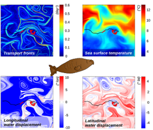
Cotté et al., 2015, analysed the behaviour of female southern elephant seals during two periods of the year: the Southern spring and the Southern summer. They evidenced that
- during the end of Southern spring (postbreeding seals), there were no environmental preference in their behaviour,
- during Southern summer (postmoult seals), they travelled along thermal fronts and foreaged in stable mesoscale waters.
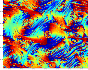
The figure opposite shows a part of an elephant trip in June/July 2005 overlaid on sub-mesoscale transport fronts (FSLE in days-1) (top,left), Sea Surface Temperature in °C (top, right), longitudinal (bottom, left) and latitudinal (bottom, right) water displacement in a 50 d backward-in-time advection at halfway through the trip part. Travelling (extensive behaviour) and foraging (intensive behaviour) bouts of trips are respectively in black and red.
References:
- Cotté C., d’Ovidio F., Dragon A.-C., Guinet C., Lévy M., 2015, "Flexible preference of southern elephant seals for distinct mesoscale features within the Antarctic Circumpolar Current", Prog. in Ocean., 131, 46–58. Available here.
Towards assimilation of images
Contrary to classical data assimilation, direct image assimilation does not work on the (mathematical) space of observed state variable (set of real numbers): discrepancy between model outputs and observations are performed in an adapted image structure space. Once defined, the image space has to be equipped with an adequate norm to measure the difference between structures (see Le Dimet et. al 2015, Titaud et al. 2010). As FSLE maps (resp. Orientations of the associated eigenvectors) show similar structures than ocean tracer images (resp. gradient of ocean tracer images), they can be used to define image observation operators: some studies have shown the great potential of this proxy data to assimilate high resolution ocean tracer image structures into meso-scale ocean model (see Gaultier et al. 2013, Titaud et al., 2011).
References:
- Le Dimet F.-X., I. Souopgui, O. Titaud, V. Shutyaev, and M. Y. Hussaini, 2015, "Toward the assimilation of images", Nonlinear Processes in Geophysics, 22(1):15--32
- Gaultier L., J. Verron, J.-M. Brankart, O. Titaud, and P. Brasseur, 2013, "On the inversion of submesoscale tracer fields to estimate the surface ocean circulation". Journal of Marine Systems, 126:33--42.
- Titaud O., J.M. Brankart, J. Verron, 2010, "On the use of Finite-Time Lyapunov Exponents and Vectors for direct assimilation of tracer images into ocean models, Tellus, 63A, 1038-1051.
Other examples of applications
A dedicated web page shows an overview of other existing studies concerning Lyapunov Exponents applications. This page will evolve based on your studies on that subject. If you are interested in a contribution to this page, feel free to contact us: aviso(at)altimetry.fr

