There are three examples below to help you manipulating the eddy files.
The examples can be downloaded here.

1: Allowing you the extraction of one eddy trajectory and store it in another file:

#!/usr/bin/env python

# -*- coding: utf-8 -*-

import xarray as xr

import numpy as np

from datetime import datetime

# Load dataset with xarray

with xr.open_dataset('eddy_trajectory_nrt_3.0exp_cyclonic_20180101_20190828.nc', decode_cf=False)  as h:
 
    lon_min, lon_max, lat_min, lat_max = 1, 5, -28, -27
    t = 25150
    # Select a specific eddy with date and area, only some observations
    subset = h.sel(obs=(h.longitude > lon_min) & (h.longitude < lon_max) & (h.latitude > lat_min) & (h.latitude < lat_max) & (h.time == 25147))
    # Extract full track
    subset = h.isel(obs=np.in1d(h.track, subset.track))
    # Store selected data
    print(subset)
    subset.to_netcdf('output_eddy.nc')

2: Allowing you plotting the selected eddy trajectory:

 

#!/usr/bin/env python
# -*- coding: utf-8 -*-
import xarray as xr
from matplotlib import pyplot as plt
# Load dataset with xarray
ax = plt.subplot(111)
with xr.open_dataset('output_eddy.nc') as h:
    N = 20
    # plot contour every N
    ax.plot((h.speed_contour_longitude[::N].T + 180) % 360 - 180, h.speed_contour_latitude[::N].T, 'r')
    # plot path
    ax.plot((h.longitude + 180) % 360 - 180, h.latitude, 'b', label='eddy path')
    ax.set_aspect('equal')
    ax.legend()
    ax.grid()
plt.show()
 
 

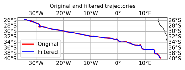
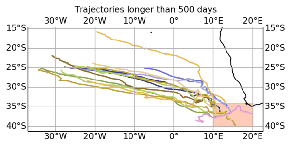
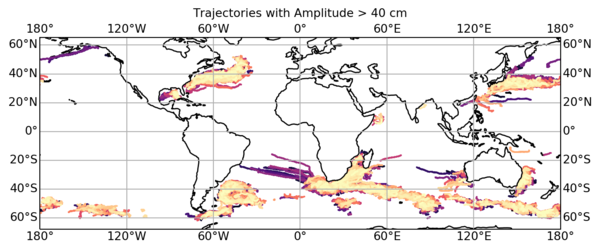
3: More advanced: Allowing you plotting a given eddy filtered track superimposed to its real track, and selecting all eddies on an area and having lifespan more than 500 days or amplitude >40cm: